Problem Statement
App wait time is the amount of time an application needs to be fully loaded. This is depicted as a cursor with a spinning wheel. The longer this cursor status is present, the longer the user must wait for the application to be fully loaded and usable. For example, Google Chrome takes an average of 10 seconds to be fully loaded up. As a result, user experience may be affected by such wait time.
In an effort to reduce app wait time, we collected data on application use and app wait time for a single user over several weeks. With this data we plan to build a series of models to predict which application the user will open with an emphasis on when and for how long. With the series of models, we will evaluate each one and select the one we think is most fitting.
Data Collection
We built upon Intel® System Usage Report (SUR), which is a framework that will be used to collect our own data for this project. This was designed to track and manage system usage in an accurate and efficient way. Intel SUR can be used to run custom input libraries (IL) to record data as needed. We will be writing custom ILs in order to collect the data that is needed for our task.
Once started, Intel® Energy Checker Energy Server (ESRV) will execute all IL and collect samples every second. If needed, a signal can be sent to collect samples so that data is only recorded as needed. Once terminated, the ESRV will stop running and write all of the data (as specified in the ILs) into a database file. For every instance that the collector is started, a new database file will be created.
Foreground Window
Many windows can be layered on top of each other, but only one window will accept input. This window is known as the Foreground Window, which was the main focus for the IL that we created. As stated above, it is important to note that the ESRV will collect samples every second, but a signal can be used instead. Knowing this, we decided to collect samples via a foreground window change. We came to this reasoning because we would end up with repeating values if the user remains on the same foreground window; this would be inefficient from a memory perspective and would make it more difficult to eventually calculate the time spent on the window. We would also lose data if the user switches foreground windows in less than a second.
We start by obtaining the handle to the foreground window and checking that the handle is valid. After obtaining the handle, we obtain the identifier of the thread that created the specified window. We then enumerate the handle in the case where we are in a child window and want to obtain the parent window. We must do so because child windows might return an executable name that does not match the true executable name. Examples of this are built-in windows applications (calculator, calendar, weather). Without enumerating, we get a return of “ApplicationFrameHost” which does not tell us anything about the executable name. Because of this, enumerating through the child windows allows us to obtain the true executable name.
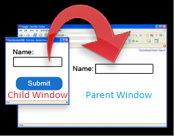
Example of Child vs. Parent Window
Now that we have the handle to the parent’s window and its identifier, we use these as parameters to obtain a handle to open this process. If we have access to this process, we can extract information from it, such as its file directory. Note that we are not opening this process with limited access, such that we will not be able to open processes that demand higher access. We are using limited access because we do not want to access sensitive information. If we are in a situation where we do not have access to open a process, we do not proceed and will simply log the output as “Admin App.”
Now that we have the file directory, we must extract only the executable name. We want to do this because we do not want to output the user’s directory, as that can obtain sensitive information.
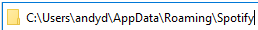
Example of File Directory
We note here that this is simply the directory for the executable. The executable will always follow this format, followed by a forward slash and then the actual executable name. In this case, the full directory will be C:\Users\andyd\AppData\Roaming\Spotify\Spotify.exe. In C, we can not simply split by a forward slash and extract the last value. Instead, we must obtain values (called tokens) for every instance of the forward slash. We continue to loop through every token until the next token is NULL. This signifies that there are no more tokens, so we simply record the last token before the NULL value. This will guarantee that we obtain the executable name and discard the previous and/or sensitive information.
As noted above, we record only when a foreground window has changed. As such, we have a variable that holds the previous executable name. Before collecting the value as a sample, we compare the previous executable name to the current one. This is because an application can have the same name, but have different process identifiers and are distinct. This can happen when an application has the ability to open up different and smaller windows, but are still connected to the main framework. The executable ‘steam.exe’ is an example because steam has smaller windows implemented, such as friends, community, trading, etc. These all will have the same parent window (steam) but will have different process identifiers. Since it has different identifiers, the ESRV will collect and log ‘steam.exe’ multiple times in a rapid succession. We want to avoid this situation because it can lead to a skewed dataset which means that our machine learning model will be less accurate. However, the use of comparing the previous executable name and the current executable name ensures that we will not run into this issue and will always log distinct values.
Dataset
Data Overview
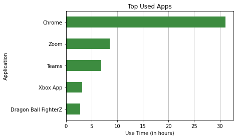
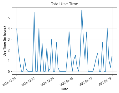
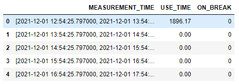
Using the data collector and input library we developed, we gathered just about 2 months worth of data from our group’s Windows 10 laptop from December 1st 2021 to January 30th 2022 over 63 collection periods. We collected foreground windows as ‘VALUE’ and recording time as ‘MEASUREMENT_TIME’. In total 68 unique applications were recorded with the most used app being Chome.
This gave us 2469 rows or foreground windows collected. This totals to about 66 hours of total active use time.
Data Cleaning
The data collector stores everything it collects into databases and separates the data into tables by data types.To extract the foreground window information we wrote a simple sql query to get all the rows for the string table. This was then converted into a Pandas dataframe and each column was changed into the correct data type as this information could be lost during conversion. Each collection session has its own database, so we did this for every session. After every dataframe was checked for errors they were merged into a larger database we would use going forward.
‘MEASUREMENT_TIME’ values were recorded in military time so we initially didn’t notice errors with this metric. However after beginning to see strange late night activity, we looked at the database files and found an inconsistency with the time the database was created and the last recording time, values that should differ by only milliseconds. Instead of using PST our collector was using UTC and we subsequently had incorrect values. This was fixed by querying the metadata table in each database to see the actual collection start time in both time zones. The difference was calculated and added to all ‘MEASUREMENT_TIME’ values in the related data.
Outliers were found after looking at the amount of time various apps were used and the unique lists of apps. Using the difference in time recorded between apps we calculated the use time for each foreground window in our dataset. Very quickly apps we were not expecting had a total use time much higher than expected. Both File Explorer and Microsoft Edge had instances where they were open for an unreasonable amount of time, which was likely the machine being left on unattended. While we do believe that these instances were not due to collector malfunction, they were removed given that their inclusion in a model could lead to unrealistic predictions based on their massive scale. We also found that in some cases the same app would have multiple names. We found both ‘Steam.exe’ and ‘steam.exe’ in our dataset and converted all app names to lowercase so future models would interpret them as the same.
Models
HMM
The first approach we tried was predicting a sequence of apps given a starting app. This would enable an underlying program to launch the predicted app in the background and decrease the wait of opening it for the user. A Hidden Markov Model (HMM) was developed for this prediction task. HMMs are statistical models that predict sequences using conditional probability, that being the odds that one event will occur given prior knowledge of another. This means that HMMs require a clear and consistent start from which all sequences start at. The HMM can visually be displayed as a decision tree, where each branch is selected based on which has the highest probability.
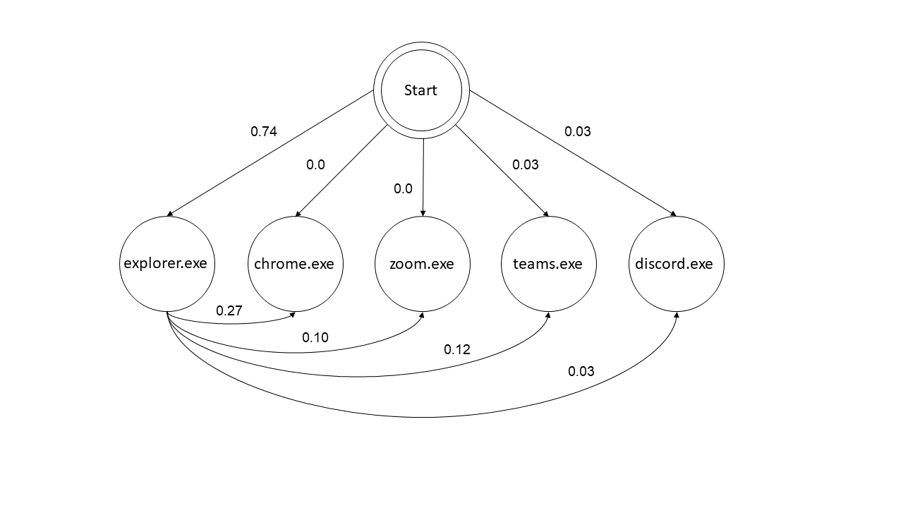
Transition Diagram for the HMM with a Selection of 5 Common Apps
For our problem we built a first order HMM, the order here refers to how much recent history is used to make individual predictions. In a first order HMM while conditional probabilities are calculated using all the training data, it’s the conditional probability based on 1 previous event. In our case that means the model knows the probability of opening Chrome given Zoom was just opened but not Chrome given two or more previous apps. While this gives the model less data, it’s much more resource efficient which is important for the eventual application. First we added a ‘s0’ app to start off each data collection period so our model could see the probability of opening each app first. The data was then split into training and test sets with 80% of observed app pairs being used for training and 20% for testing. Training consisted of creating a (n x n) transition matrix where n is the number of apps in the training set. For a position of the matrix (A, B) it contains the conditional probability of opening app A given app B calculated by:
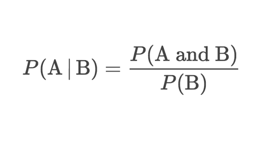
These probabilities were further verified by making sure the rows of the transition matrix summed to 1 as that would represent all possibilities of A.
Using this matrix the model would predict a sequence of apps given a desired sequence length and starting app which defaulted to ‘s0’. Ultimately when predicting just the following app, so a sequence of 2, the model had an accuracy of only 17%. This is due to several factors. Firstly, the data was unbalanced. The user spent a disproportionate amount of time using a small sample of apps, so those used most would be predicted much more than they actually appeared in the data. There also was low dimensionality so the model had less history to work with and was essentially forgetful, therefore it needed to have more past data to accurately predict for our dataset. Lastly, for this approach we had too many apps. With over 50 apps there aren’t a lot of possible predictions with unequal amounts of data. This made us consider lowering our scope to one app at a time.
LSTM
Understanding we would likely need to narrow our focus and increase memory retention in our model to improve results, we moved on to our second approach. This time we predicted the use time of a single app within a given hour. This would allow a user to have apps preloaded as well but would require more models (one for each app) at the benefit of more accurate predictions. A Long Short Term Memory Recurrent Neural Network (LSTM RNN) was used in this problem. The LSTM in the name refers to a cell type in the network that improves accuracy by strengthening long-term and working memory. This type of model is a great predictor for time series problems because of how it learns from the entire training series, rather than pairs, for predictions.
Before creating our LSTM, we first had to encode our data in such a way that the model can use it as inputs. Our initial approach was to bin the use time by hour in each row, and to measure the seconds in each hour Google Chrome was used. We chose to analyze Google Chrome because this was our most used app, thus having the most data. This means that we will get a larger dataset if we were to filter the dataset with only one application. Our other apps did not have sufficient data to be used in this model. Our Google Chrome dataset had 2 features, with the columns being USE_TIME, the use time for Google Chrome in seconds during the hour, and on break, a feature that denotes whether the user was using the machine during a time that school was not in session. The rows in this dataset were split by the hour, ranging from the first hour when data was successfully recorded to the last hour that the ESRV was running.
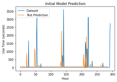
A high accuracy was achieved with our LSTM (specifically 96%) but after further investigation, this was because of the model predicting only one value. Since most of the use times within our data were 0s, it made sense on why the model only predicted one value. The LSTM did not capture the peaks and we were not sure why this was happening. We wanted to build upon this prototype, and make it as best as we can.
Before making any major changes to our model, specifically the encoding of our data, we opted to look at our accuracy metric and adjust the hyperparameters of our model. After looking into how our model dealt with accuracy, we discovered that our model was overestimating in order to achieve a high score in that category. This was not what we wanted as an indicator as to how good our model was doing, as estimating an exact use time in our use case would be extremely hard. Instead, we opted to create our own accuracy metric, which instead would use a range instead of an exact value. True would only be returned, given that the predicted value landed in a range relative to the actual value. The default range was ± .5 * the actual value, but this was easily adjustable from the parameters of the function. We also noticed that some models would predict very small values for 0 that would vary every time the model was re-trained. From a human eye it was clear these functioned as 0’s as they would be consistent with the zeroes in our data. To make sure our accuracy metric captured this, the outputs would be subtracted by that model’s zero value.
Next, we looked into the hyperparameters of the model and tinkered with them until we got a result that we were satisfied with. One hyperparameter was focused at a time, with each one being manually changed to achieve best performance. We adjusted one hyperparameter until it could not get any better, then moved on to the next one. Our edited hyperparameters were with 5 layers, a batch size of 2, and a lookback value of 3. We then incorporated a new method when dealing with the last two hyperparameters, the loss function and optimizer. Since these two hyperparameters had a finite amount of choices, we ran them in a nested for loop to see which combination of the two gave us the best choice. 56 models were run, and the results of 5 are listed in the table below.
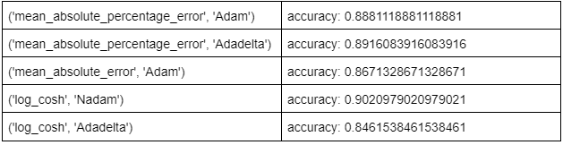
As you can see, the results varied a lot and we couldn’t tell which of the models did the best. We first took a look at the combinations with a 96% or higher accuracy calculated using the model’s function. Despite their accuracy being good, we were still skeptical of the high values and started looking at them through our own accuracy metric. Even with this new perspective, results still varied and there was still a lot of overestimation. Our next step was to review these models visually, and the best one to us was the one with the logcosh loss function and the NAdam optimizer. Not only did it boast a 90% accuracy with our own function, this model actually tried to capture some of the peaks within our dataset, and did not fall back to overestimating the predictions. This was our best model yet, and it resembled the dataset even more than the previous one did. We still wanted to further optimize this model, and turned to changing the encoding of our dataset.
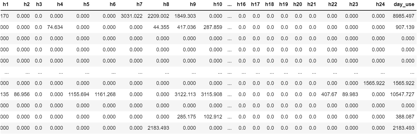
Since the previous LSTM only had 2 input columns with our dataset, our next goal was to add more features for the model to use. Instead of having just 2 features, we revised it to have 24, which represented the seconds used in an hour of the day. We had an additional 25th label column which showed the total seconds Google Chrome was used in a 24 hour instance. For our rows, each one represented a day in which data was recorded. In total, we had 61 rows worth of data, and 24 columns as inputs.
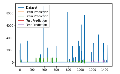
With our new encoding, we were ready to run the model and see our results. Unfortunately, we had to change much of our previous code on how we ran the model and graphed it, as it was catered to our 2 feature dataset. This took more time than expected, so most default hyperparameters were used, with the loss function being mean squared error and the optimizer being Adam. The only change we made to the hyperparameters was changing epochs to 400, as this model took longer for the loss to converge.
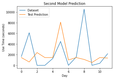
As you can see here, our new inputs did not perform as we wanted it to, and actually resulted in a worse accuracy than our previous model. This one ended with an accuracy of 33%, which was 67% lower than our previous model. Despite our best attempts, this was the end result of our last modification given our allotted time. However, we were not discouraged by this result, as visually, you can see how this model tried harder to capture peaks and prevent overestimating. Many more ideas were thought of to improve our model and finally reach our end goal in the near future.
Discussion
Limitations
During the initial state of data collection, we ran into multiple obstacles that we had to overcome. First of all, we did not perfect our other input library (Desktop Mapper) for it to collect other metrics in relation to the foreground window. Before starting the data collection period, we only ended up with just using one input library to record the foreground window executable and its use time. To make matters worse, we only had one laptop to record data off of, which required the user to be constantly be using this machine, thus hindering the amount of data we have. Instead of crippling ourselves and using only those metrics for our model, we expanded upon it and added more features for the model to be trained on. ON_BREAK is an example of a feature we added that was not part of the data collection process. We insisted on adding this to explain the big spikes in our data, in which it definitely improved our results. We also tried modifying the dataset in a way that resulted in multiple features, as seen in our last optimization which included 25 columns instead of the original 2.
Our biggest struggle was with coding in the language of C. Our group was not comfortable coding in C, as all of us were only accustomed to mainly doing things in Python. However, we took a different perspective on this, and saw it as a challenge we had to overcome. We saw this as an opportunity to get better at coding in C, and to also learn the intricacies of the language since this was opted over Python. C had to be utilized in such a way that while collecting data, the user was unobstructed and that their privacy was not at risk. Because of these two factors, we were limited on how much of the user’s data we could access. Using resources such as SUR and ESRV documentation, we managed to create a data collector with the use of C and Intel libraries, while keeping in mind the memory usage and privacy.
Future Plans
Despite so much progress on this project, there is actually much more that we can do to finally reach our end goal of predicting a user’s next open app and preloading it in the background. First of all, we can add more features to our data collector by creating and finishing up more input libraries. With this new information, we can feed more information to our model, thus resulting in more features and potentially better predictions. Once we get the model to a point we are comfortable with, the LSTM can be expanded upon just predicting just one app, and predict use time for multiple apps in the same timeframe. This can lead us into also predicting the next app opened, which is essential to what our original goal is, to preload apps. And finally, we can get to the point where we actually preload the app and improve the user’s experience on their machine.
Conclusion
To conclude, we were able to construct a data collector using the Intel® System Usage Report and our own input libraries to collect the foreground data of a user’s machine without slowdown. With this data, a LSTM model was created and used to predict the use time of the app Google Chrome with moderate accuracy. Our goal of predicting the next application that would be used was not reached, but upon expanding on this model and its features, this could be worked up to.